"1 Color Looks like 2". Palette found using optimization over inputs to DDIM inversion. Hover/Tap to see visual proof that the squares are indeed the same color.

the relativity of color

In visual perception a colour is almost never seen as it really is - as it physically is. This fact makes colour the most relative medium in art...

In order to use color effectively it is necessary to recognize that color deceives continually. The aim of such study is to develop—through experience—by trial and error—an eye for color. This means, specifically, seeing color action as well as feeling color relatedness.

Josef Albers, Interaction of Color, 1963¹

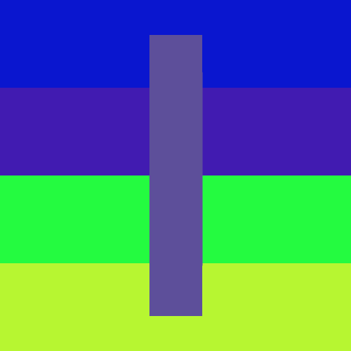
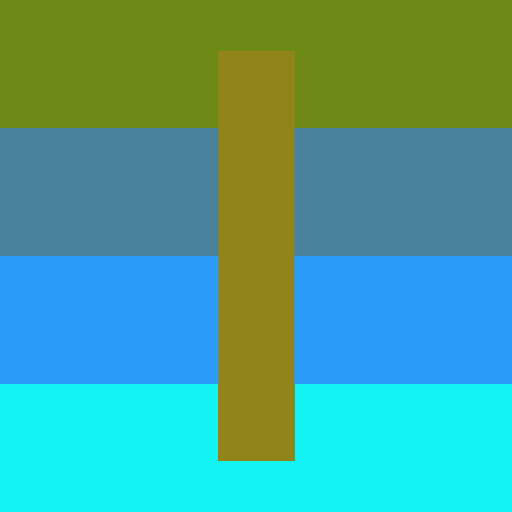
Albers demonstrates this concept through a set of simple experiments called plates, such as placing two identical colors on different backgrounds, which causes the colors to appear different due to the influence of their surroundings. This phenomenon is known as simultaneous contrast or chromatic induction, in which adjacent colors exert influence on each other, altering their perceived hue, value, and saturation.²

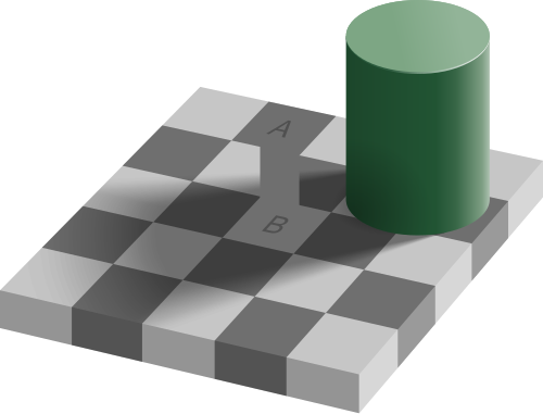
Note that this is related but different from color / lightness constancy, in which the perceived color or lightness of an object remains relatively constant under varying illumination conditions. A common visual illusion that exploits color constancy is the checker shadow illusion, in which two squares of identical color appear different due to the context of shadows and surrounding colors. Simultaneous contrast is perhaps a local manifestation of this phenomenon between adjacent colors.

Example of color constancy. One color looks like two due to the context of shadows.³

At the heart of Albers' experiments is a pedagogical approach that lets us experience and learn what colors lead to certain perceptual effects. For instance, what combinations of square and background colors make the square look most different when placed on different backgrounds? Certain color combinations lead to stronger contrast effects, while others lead to weaker effects. Another exercise might be to find color combinations that result in two different colors looking the same when placed on different backgrounds. Lastly, using this understanding, how can we create more effective designs and artworks that leverage contrast?

Certain combinations of colors result in squares that appear the same (left). Other combinations result in squares that look completely different despite being the same color (right). All generated with optimization over inputs to DDIM inversion.

Interestingly, it appears that diffusion models have learned some of those lessons. Not from Albers, but from the statistics of natural images. And we can surface those lessons by optimizing over the model's inputs.

visual illusions as learned natural priors

Gomez-Villa et al. show that visual illusions learned by diffusion models align well with human perception.⁴ They suggest that natural images have statistical regularities brought on by the physics of light affecting the illumination and thus the local color of an object (color and light constancy). Perhaps the learned model internalizes these patterns as part of its learned data distribution.

For example, if a natural photograph contains a medium-gray object surrounded by deep, dark shadows, that object is likely a bright object in a dark scene. If the exact same object is surrounded by blinding white light, it is more likely to be a dark object.

When we feed the model an image of two identical squares on different backgrounds, the model's learned priors make it predict different "true" colors when corrupted by moderate noise levels.

diffusion models and simultaneous contrast

In the forward diffusion process, we gradually corrupt a clean image \( x_0 \) by adding Gaussian noise. The marginal distribution at timestep \( t \) is given by: $$ q(x_t | x_0) = \mathcal{N}(x_t; \sqrt{\bar{\alpha}_t} x_0, (1 - \bar{\alpha}_t) I) $$ Using the reparameterization trick, we can sample \( x_t \) directly: $$ x_t = \sqrt{\bar{\alpha}_t} x_0 + \sqrt{1 - \bar{\alpha}_t} \epsilon, \epsilon \sim \mathcal{N}(0, I)$$ Where \( \bar{\alpha}_t \) is a noise schedule that controls the amount of noise added at each timestep.

Note that this forward corruption is entirely independent per-pixel: the covariance matrix is purely diagonal. If we have two identical center squares on different backgrounds, the physical noise added to each square is statistically identical.

The reverse process learns a neural network \( \epsilon_\theta(x_t, t) \), to predict the injected noise at time \( t \). Through the lens of score-matching, predicting this noise is equivalent to approximating the score function of the noised data distribution at time \( t \): $$ \epsilon_\theta(x_t, t) \approx -\sqrt{1 - \bar{\alpha}_t} \nabla_{x_t} \log p(x_t) $$ Note that \( p(x_t) \) is the joint distribution of all pixels in our dataset (ideally the distribution of all natural images) at noise level \( t \). Consequently, the score and thus the learned prediction for a specific pixel \( x_t^{(i)} \) is a function of the entire image context \( x_t^{(-i)} \).

Thus, despite the forward process adding independent noise to each pixel, the reverse process does not treat each pixel independently. As a consequence, the noise prediction for identical pixels will differ based on the background context. Since the pixel values are identical in the clean image and the noise added during the forward process was independent, the learned reconstruction can only differ due to the influence of the background context biasing the learned score function.

ddim inversion as an ode

Denoising Diffusion Implicit Model (DDIM) formulates sampling from a diffusion model as solving an ordinary differential equation (ODE) in the latent space of the model.

Because it is deterministic, we can invert a real image \( x_0 \) back into the latent representation \( x_T \) that would generate it. This latent representation \( x_T \) is influenced by the learned score function: $$ x_{t+1} = \sqrt{\bar{\alpha}_{t+1}} \underbrace{\left( \frac{x_t - \sqrt{1-\bar{\alpha}_t}\epsilon_\theta(x_t, t)}{\sqrt{\bar{\alpha}_t}} \right)}_{\text{predicted } x_0} + \sqrt{1-\bar{\alpha}_{t+1}}\epsilon_\theta(x_t, t) $$
As we integrate this ODE over time, the contextual differences in the score function \( \epsilon_\theta \) accumulate. The latent representations of the two initially identical squares drift apart in the latent space. Gomez-Villa et al. demonstrated that this drift aligns well with human optical illusions, which in turn makes diffusion models "susceptible" to the same visual illusions as humans.⁴

We can feed different illusions into the inverted DDIM process and see how far the values for identical pixels drift apart during inversion, which gives us a quantitative measure of how strongly the model perceives the illusion.

optimizing for simultaneous contrast

We can repurpose this measure as an objective function to solve a classic pedagogical exercise: finding palettes for Albers' plates.

As latents drift apart during DDIM inversion, decoding them back into pixel space at different noise levels \( t \) will result in different perceived colors for the center square. We can optimize for color combinations that maximize this perceptual difference, effectively learning which colors lead to stronger simultaneous contrast effects according to the model's learned priors.

Let an image \( I \) be composed of a square color \( c_s \) and some background colors \( \vec c_b \), defined using a spatial mask \( M \): $$ I(c_s, \vec c_b) = M \odot c_s + (1 - M) \odot \vec c_b $$ We seek to find the color palette \( \{c_s, \vec c_b\} \) that maximizes the perceptual difference of the square colors after inversion. Let \( f_\theta(I) \) denote the mapping of an image through DDIM inversion up to timestep \( T \). Our objective function is: $$ \arg\max_{c_s, \vec c_b} \mathcal{D}\Big( M \odot f_\theta(I(c_s, c_{b1})), \; M \odot f_\theta(I(c_s, c_{b2})) \Big) $$ where \( \mathcal{D} \) is a distance metric (e.g., \( L_2 \) distance in the latent space or, more accurately, predict the clean image in pixel space at the current noise level \( \hat I_0(x_t) \) and measure perceptual distance using a metric like CIEDE2000. The images in this post along with the source code below use the latter).

While we could theoretically compute the gradient of this objective with respect to the input colors, backpropagating through the unrolled ODE solver (e.g., 50 sequential forward passes of Stable Diffusion's U-Net) is not for the GPU poor.

Instead, we can treat stable diffusion as a black-box and run a zeroth-order optimization problem over a continuous search space \( \mathcal{X} \subset [0, 1]^{3N} \) representing the RGB channels of \( c_s \) and \(N-1\) background colors. I chose Gaussian Process (GP) Optimization, which builds a surrogate model of the objective landscape, mainly because it's quite sample-efficient, which is nice because stable diffusion inference is still kind of expensive.

Example palette found by optimization over inputs to DDIM inversion. Hover/Tap to see visual proof that the squares are indeed the same color.

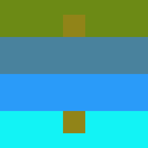
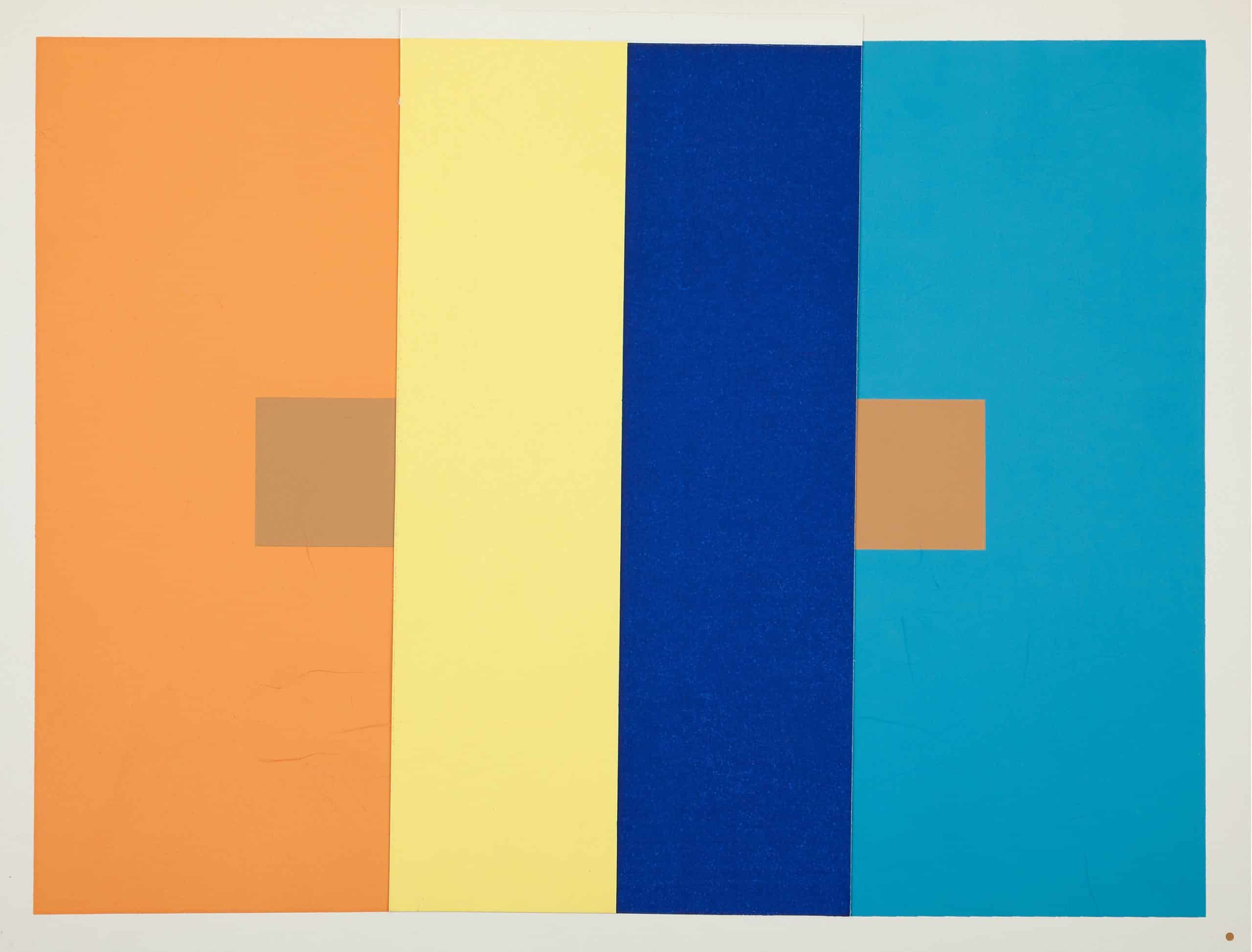
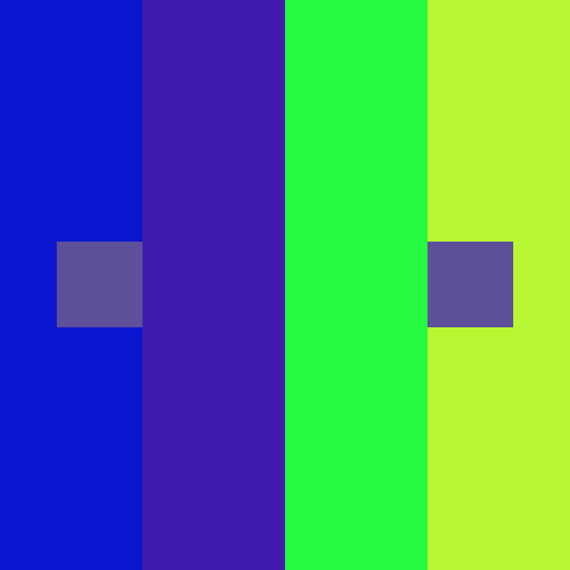
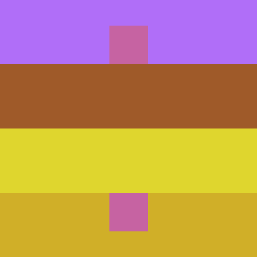
From the generated images, the optimization tends to put one of the squares on top of a background of similar hue, which maximizes the brightness contrast and makes the square appear lighter or darker. The optimization also seems to prefer putting the other square on top of a complementary color, which may enhance the hue contrast and thus further strengthen the effect. For instance, the first image on the left has a purple square on top of a highly saturated, slightly darker blue, and the other purple square on a bright yellow-green background.

Interestingly, this trend actually matches Albers' original palette for this particular plate design: orange squares on top of a similar, slightly brighter orange and a sky blue (complementary) background.

It's true, asking AI to produce these palettes nullifies Albers' emphasis on developing an eye for color through our own, human, trial-and-error experience. Oops. The most useful lesson would still be to find these palettes through patient experimentation and some reflections on color theory. But it's interesting to see that a pretrained model and a few function evaluations can get us there too.

source code and procedure

1. Sample a color palette \( \{c_s, \vec c_b\} \) and compose the desired plate \( I \).
2. Run DDIM inversion to some timestep \( t \), predict the clean image \( \hat I_0 \), and compute the perceptual difference objective.
3. Update the surrogate model with the new data point.
4. Run optimization on the surrogate model to propose a new color palette to evaluate on the true objective.
5. Repeat steps 1-4 a few times until convergence.

references

1. Albers, J. (1963). Interaction of Color. Yale University Press.
2. https://en.wikipedia.org/wiki/Contrast_effect
3. https://en.wikipedia.org/wiki/Checker_shadow_illusion
4. Gomez-Villa, A., et al. “The Art of Deception: Color Visual Illusions and Diffusion Models.” CVPR, 2025, https://arxiv.org/abs/2412.10122.